Worldclim data with R: the right way
Introduction
Worldclim data is a great source of environmental data opensource data. Its a database of high spatial resolution global weather and climate data. Worldclim (Fick and Hijmans, 2017) is in its version 2.1 and it has climate data from 1970 to 2000. Containing several bioclimatic variables derived from monthly temperatre and rainfall values, the data is usually applied to ecology and modelling techniques. Although you can download all the data here, Worldclim data can also be easily downloaded using the raster package with R using few lines of code.
This approach will, however , soon be deprecated due to the retirement of rgdal, rgeos and maptools. Hopefully, Worldclim is still easlly acessible. For this post, we will focus on how to extract and plot data from Worldclim, focusing on preciptation raster in Nigeria
The right way
Any user with litte experience with R may quickly acess the worldclim large set of raster files containing many environmental data. With the deprecation rdal and others, wordclim is managed by the geodata package. Depending on your R versiom, you might still be able to run raster and rgal packages, but its very likelly will you find some warnings. Plus, it is better to get used to the new practices of spatial data manipulation in R, that is, the use of the sf package. Let’s start !
Set raster and vector path
We start by defining raster and vector paths. For raster data, you can set raster_path = tempdir() if you want to download the data into a temp folder. If not, set it to folder of preference. You can also do the same for vector_output_path.
raster_path_folder = tempdir()
vector_output_path = "~/nigeria_adm2"
vector_output_file = paste0(vector_output_path, ".zip")
Load data from worldclim
Now, we use a worlclim function called worldclim_country. The res paramater is the resolution, with valid values as 10,5,2.5 and 0.5. The var parameter is the variable name, with valid values as tmin, tmax, tavg, prec, wind,
vapr and bio.
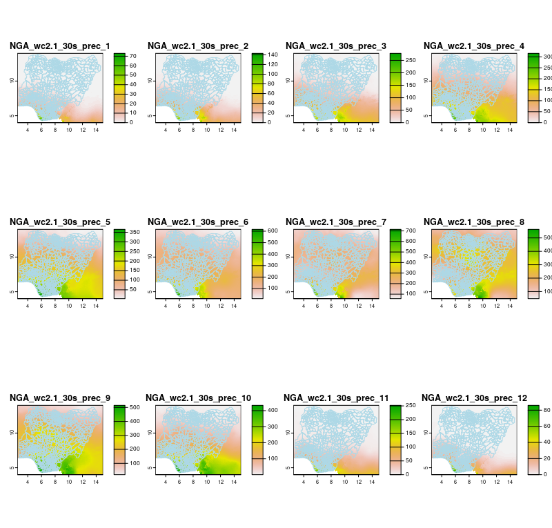
Using the code bellow, we chose prec since we are interested in precipitation data. Thus, the worldclim_country function will return 12 layers of raster (in a raster stack), each image representing a month of precipitation in Nigeria (NGA). We later save the coordinate system of the data for later use in line 2
raster_stack <- worldclim_country(country = "NGA",path = raster_path_folder ,version="2.1",res=0.5,var="prec")
crs_proj <- crs(raster_stack)
Download the shapefile
You can manually download and extract data from the OCHC site. The nigeria administrative level 2 vector data is avaiable here. Or, you can just run these two lines :
download.file("https://data.humdata.org/dataset/aac2a1d6-36c6-4f47-beee-34415742180d/resource/d7011402-0a22-4927-82eb-1359d17ff5cd/download/nigeria_admin_level_2.zip" , destfile=vector_output_file)
unzip(vector_output_file, exdir = vector_output_path)
Read the downloaded shape file
If we want to plot them together, we must be sure that they belong to the same coordinate system. Let’s apply the coordinate systems saved previously in crs_proj and apply it to the nigeria admin level boundaries
nigeria_vector_adm2 <- read_sf(paste0(vector_output_path,"/","Nigeria_Admin_Level_2.shp"))
nigeria_vector_adm2 <- st_transform(nigeria_vector_adm2, st_crs(raster_stack))
All we have to do now is to set the plot to 12 subplots, using the par function, loop over the raster stack and plot nigeria boundaries.
# Set up plot area
par(mfrow=c(3,4))

# Loop layers and plot
for (i in 1:length(raster_stack[1])){
  plot(raster_stack[[i]], main=names(raster_stack[[i]]))
  plot(st_geometry(nigeria_vector_adm2),bg='transparent', border = "lightblue", add=T)
}
And the result :

References
Fick, S.E., Hijmans, R.J., 2017. WorldClim 2: new 1-km spatial resolution climate surfaces for global land areas. International Journal of Climatology 37, 4302–4315. https://doi.org/https://doi.org/10.1002/joc.5086